文章目录
- Highway-env Intersection
- rl-agents之DQN
- *Implemented variants*:
- *References*:
- Query agent for actions sequence
- 探索策略
- 神经网络实现
- 小结1
- Record the experience
- Replaybuffer
- compute_bellman_residual
- step_optimizer
- update_target_network
- 小结2
- exploration_policy
- Greedy
- ϵ \epsilon ϵ-Greedy
- Boltzmann
- 运行结果
Highway-env Intersection
本文将继续探索rl-agents中相关DQN算法的实现。下面的介绍将会以intersection这个环境为例,首先介绍一下Highway-env中的intersection-v1。Highway-env中相关文档——http://highway-env.farama.org/environments/intersection/。
highway-env中的环境可以通过配置文件进行修改, observations, actions, dynamics 以及rewards等信息都是以字典的形式存储在配置文件中。
PS:DQN、DuelingDQN算法原理可参考【强化学习】10 —— DQN算法【强化学习】11 —— Double DQN算法与Dueling DQN算法
import gymnasium as gym
import pprint
from matplotlib import pyplot as plt

env = gym.make("intersection-v1", render_mode='rgb_array')
pprint.pprint(env.unwrapped.config)
输出config,可以看到如下信息:
{'action': {'dynamical': True,
            'lateral': True,
            'longitudinal': True,
            'steering_range': [-1.0471975511965976, 1.0471975511965976],
            'type': 'ContinuousAction'},
 'arrived_reward': 1,
 'centering_position': [0.5, 0.6],
 'collision_reward': -5,
 'controlled_vehicles': 1,
 'destination': 'o1',
 'duration': 13,
 'high_speed_reward': 1,
 'initial_vehicle_count': 10,
 'manual_control': False,
 'normalize_reward': False,
 'observation': {'features': ['presence',
                              'x',
                              'y',
                              'vx',
                              'vy',
                              'long_off',
                              'lat_off',
                              'ang_off'],
                 'type': 'Kinematics',
                 'vehicles_count': 5},
 'offroad_terminal': False,
 'offscreen_rendering': False,
 'other_vehicles_type': 'highway_env.vehicle.behavior.IDMVehicle',
 'policy_frequency': 1,
 'real_time_rendering': False,
 'render_agent': True,
 'reward_speed_range': [7.0, 9.0],
 'scaling': 7.15,
 'screen_height': 600,
 'screen_width': 600,
 'show_trajectories': False,
 'simulation_frequency': 15,
 'spawn_probability': 0.6}
之后可以通过以下代码输出图像:
plt.imshow(env.render())
plt.show()

输出observation,可以看到是一个5*8的array,:
[[ 1.0000000e+00  9.9999998e-03  1.0000000e+00  0.0000000e+00
  -1.2500000e-01  6.3297665e+01  0.0000000e+00  0.0000000e+00]
 [ 1.0000000e+00  1.3849856e-01 -1.0000000e+00 -9.9416278e-02
   1.2500000e-01  8.1300293e+01  1.0361128e-15  0.0000000e+00]
 [ 1.0000000e+00 -2.0000000e-02 -1.0000000e+00  0.0000000e+00
   2.2993930e-01  6.5756187e+01  2.8473811e-15  0.0000000e+00]
 [ 0.0000000e+00  0.0000000e+00  0.0000000e+00  0.0000000e+00
   0.0000000e+00  0.0000000e+00  0.0000000e+00  0.0000000e+00]
 [ 0.0000000e+00  0.0000000e+00  0.0000000e+00  0.0000000e+00
   0.0000000e+00  0.0000000e+00  0.0000000e+00  0.0000000e+00]]
observation的解释如下,

通过以下代码,可以将action的类型变为离散的空间。
env.unwrapped.configure({
    "action": {
        'longitudinal': True,
        "type": "DiscreteMetaAction"
    }
})
rl-agents之DQN
A neural-network model is used to estimate the state-action value function and produce a greedy optimal policy.
Implemented variants:
- Double DQN
- Dueling architecture
- N-step targets
References:
Playing Atari with Deep Reinforcement Learning, Mnih V. et al (2013).
Deep Reinforcement Learning with Double Q-learning, van Hasselt H. et al. (2015).
Dueling Network Architectures for Deep Reinforcement Learning, Wang Z. et al. (2015).
Query agent for actions sequence
由上一节所知,通过调用run_episodes函数,进行具体的agent训练。其中会调用step函数,并执行self.agent.plan(self.observation)。对于DQNAgent的实现,首先由AbstractAgent类实现plan,之后plan函数会调用act函数:
    def step(self):
        """
            Plan a sequence of actions according to the agent policy, and step the environment accordingly.
        """
        # Query agent for actions sequence
        actions = self.agent.plan(self.observation)
// rl_agents/agents/common/abstract.py
class AbstractAgent(Configurable, ABC):

    def __init__(self, config=None):
        super(AbstractAgent, self).__init__(config)
        self.writer = None  # Tensorboard writer
        self.directory = None  # Run directory

    @abstractmethod
    def act(self, state):
        """
            Pick an action

        :param state: s, the current state of the agent
        :return: a, the action to perform
        """
        raise NotImplementedError()

    def plan(self, state):
        """
            Plan an optimal trajectory from an initial state.

        :param state: s, the initial state of the agent
        :return: [a0, a1, a2...], a sequence of actions to perform
        """
        return [self.act(state)]
DQN抽象类AbstractDQNAgent继承自AbstractStochasticAgent,AbstractStochasticAgent继承自AbstractAgent,在DQN抽象类AbstractDQNAgent中实现对act函数的重写:
    def act(self, state, step_exploration_time=True):
        """
            Act according to the state-action value model and an exploration policy
        :param state: current state
        :param step_exploration_time: step the exploration schedule
        :return: an action
        """
        self.previous_state = state
        if step_exploration_time:
            self.exploration_policy.step_time()
        # Handle multi-agent observations
        # TODO: it would be more efficient to forward a batch of states
        if isinstance(state, tuple):
            return tuple(self.act(agent_state, step_exploration_time=False) for agent_state in state)

        # Single-agent setting
        values = self.get_state_action_values(state)
        self.exploration_policy.update(values)
        return self.exploration_policy.sample()
探索策略
首先来看一下exploration_policy 的实现:
self.exploration_policy = exploration_factory(self.config["exploration"], self.env.action_space)
探索策略加载的配置文件部分:
"exploration": {
 "method": "EpsilonGreedy",
    "tau": 15000,
    "temperature": 1.0,
    "final_temperature": 0.05
}
跳转到exploration_factory,可以看到主要实现了三类探索策略,具体的内容会在后面部分进行介绍:
- Greedy
- ϵ \epsilon ϵ-Greedy
- Boltzmann
def exploration_factory(exploration_config, action_space):
    """
        Handles creation of exploration policies
    :param exploration_config: configuration dictionary of the policy, must contain a "method" key
    :param action_space: the environment action space
    :return: a new exploration policy
    """
    from rl_agents.agents.common.exploration.boltzmann import Boltzmann
    from rl_agents.agents.common.exploration.epsilon_greedy import EpsilonGreedy
    from rl_agents.agents.common.exploration.greedy import Greedy

    if exploration_config['method'] == 'Greedy':
        return Greedy(action_space, exploration_config)
    elif exploration_config['method'] == 'EpsilonGreedy':
        return EpsilonGreedy(action_space, exploration_config)
    elif exploration_config['method'] == 'Boltzmann':
        return Boltzmann(action_space, exploration_config)
    else:
        raise ValueError("Unknown exploration method")
神经网络实现
接着获取 Q ( s , a ) Q(s,a) Q(s,a)值
    def get_state_action_values(self, state):
        """
        :param state: s, an environment state
        :return: [Q(a1,s), ..., Q(an,s)] the array of its action-values for each actions
        """
        return self.get_batch_state_action_values([state])[0]
调用了抽象方法get_batch_state_action_values
    @abstractmethod
    def get_batch_state_action_values(self, states):
        """
        Get the state-action values of several states
        :param states: [s1; ...; sN] an array of states
        :return: values:[[Q11, ..., Q1n]; ...] the array of all action values for each state
        """
        raise NotImplementedError
接着来看DQNAgent中的具体实现:
class DQNAgent(AbstractDQNAgent):
    def __init__(self, env, config=None):
        super(DQNAgent, self).__init__(env, config)
        size_model_config(self.env, self.config["model"])
        self.value_net = model_factory(self.config["model"])
        self.target_net = model_factory(self.config["model"])
        self.target_net.load_state_dict(self.value_net.state_dict())
        self.target_net.eval()
        logger.debug("Number of trainable parameters: {}".format(trainable_parameters(self.value_net)))
        self.device = choose_device(self.config["device"])
        self.value_net.to(self.device)
        self.target_net.to(self.device)
        self.loss_function = loss_function_factory(self.config["loss_function"])
        self.optimizer = optimizer_factory(self.config["optimizer"]["type"],
                                           self.value_net.parameters(),
                                           **self.config["optimizer"])
        self.steps = 0

    def get_batch_state_action_values(self, states):
        return self.value_net(torch.tensor(states, dtype=torch.float).to(self.device)).data.cpu().numpy()
value_net的实现依赖于model_factory,其中的配置文件部分如下:
    "model": {
        "type": "MultiLayerPerceptron",
        "layers": [128, 128]
    },
再进入model_factory,主要实现了四类网络:
- MultiLayerPerceptron
- DuelingNetwork
- ConvolutionalNetwork
- EgoAttentionNetwork
这里我们暂且先分析多层感知机MultiLayerPerceptron(即普通DQN)。
// rl_agents/agents/common/models.py
def model_factory(config: dict) -> nn.Module:
    if config["type"] == "MultiLayerPerceptron":
        return MultiLayerPerceptron(config)
    elif config["type"] == "DuelingNetwork":
        return DuelingNetwork(config)
    elif config["type"] == "ConvolutionalNetwork":
        return ConvolutionalNetwork(config)
    elif config["type"] == "EgoAttentionNetwork":
        return EgoAttentionNetwork(config)
    else:
        raise ValueError("Unknown model type")
MultiLayerPerceptron类继承自BaseModule,BaseModule继承自torch.nn.Module。根据配置文件baseline.json,可以看到MultiLayerPerceptron类的sizes为[128, 128],激活函数为RELU。我们可以注意到,网络实现中有reshape操作,因为state的输入是5*8的矩阵,通过reshape,可以将其转换为一维的向量。最终网络结构类似于下图。

class MultiLayerPerceptron(BaseModule, Configurable):
    def __init__(self, config):
        super().__init__()
        Configurable.__init__(self, config)
        sizes = [self.config["in"]] + self.config["layers"]
        self.activation = activation_factory(self.config["activation"])
        layers_list = [nn.Linear(sizes[i], sizes[i + 1]) for i in range(len(sizes) - 1)]
        self.layers = nn.ModuleList(layers_list)
        if self.config.get("out", None):
            self.predict = nn.Linear(sizes[-1], self.config["out"])

    @classmethod
    def default_config(cls):
        return {"in": None,
                "layers": [64, 64],
                "activation": "RELU",
                "reshape": "True",
                "out": None}

    def forward(self, x):
        if self.config["reshape"]:
            x = x.reshape(x.shape[0], -1)  # We expect a batch of vectors
        for layer in self.layers:
            x = self.activation(layer(x))
        if self.config.get("out", None):
            x = self.predict(x)
        return x
获取
Q
Q
Q之后,探索策略进行更新,并sample一个action。以
ϵ
\epsilon
ϵ-Greedy为例,因为
ϵ
\epsilon
ϵ-Greedy继承DiscreteDistribution,所以主要关注DiscreteDistribution中的相关实现。
    def act(self, state, step_exploration_time=True):
    ...
        self.exploration_policy.update(values)
        return self.exploration_policy.sample()
rl_agents/agents/common/exploration/epsilon_greedy.py
    def update(self, values):
        """
            Update the action distribution parameters
        :param values: the state-action values
        :param step_time: whether to update epsilon schedule
        """
        self.optimal_action = np.argmax(values)
        self.epsilon = self.config['final_temperature'] + \
            (self.config['temperature'] - self.config['final_temperature']) * \
            np.exp(- self.time / self.config['tau'])
        if self.writer:
            self.writer.add_scalar('exploration/epsilon', self.epsilon, self.time)
class DiscreteDistribution(Configurable, ABC):
    def __init__(self, config=None, **kwargs):
        super(DiscreteDistribution, self).__init__(config)
        self.np_random = None

    @abstractmethod
    def get_distribution(self):
        """
        :return: a distribution over actions {action:probability}
        """
        raise NotImplementedError()

    def sample(self):
        """
        :return: an action sampled from the distribution
        """
        distribution = self.get_distribution()
        return self.np_random.choice(list(distribution.keys()), 1, p=np.array(list(distribution.values())))[0]
可以看到首先需要获得action的一个分布,这部分在 ϵ \epsilon ϵ-Greedy中的实现为:
    def get_distribution(self):
        distribution = {action: self.epsilon / self.action_space.n for action in range(self.action_space.n)}
        distribution[self.optimal_action] += 1 - self.epsilon
        return distribution
get_distribution 函数返回一个动作的概率分布字典。字典的键是动作,字典的值是动作被选择的概率。概率分布的计算方式为:每个动作都有一个基础概率 self.epsilon / self.action_space.n,其中 self.action_space.n 是动作的总数,即每个动作被选择的概率相等,这是基于探索的角度。同时,最优动作 self.optimal_action 会额外获得一个概率增量 1 - self.epsilon,这是基于利用的角度,即利用已知的最优动作。
sample 函数根据 get_distribution 函数得到的动作概率分布进行采样,返回一个动作。具体地,使用 np_random.choice 函数,其参数包括动作列表和对应的动作概率分布列表,返回的是一个根据给定概率分布随机采样的动作。
小结1
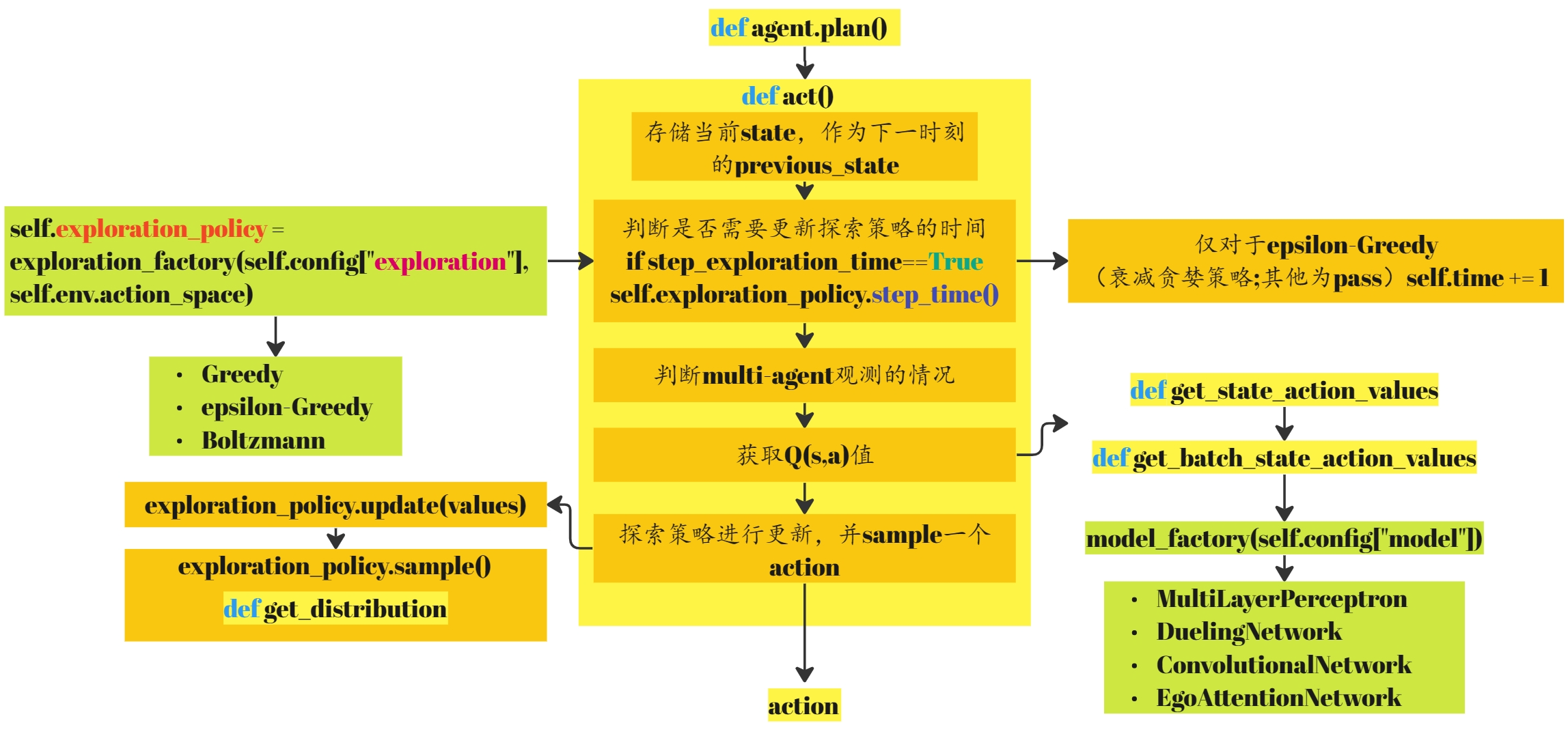
到此,act函数返回一个待执行的action,此部分的框图如下所示:
之后这几步在上一讲已经讨论过http://t.csdnimg.cn/ddpVJ。
        # Forward the actions to the environment viewer
        try:
            self.env.unwrapped.viewer.set_agent_action_sequence(actions)
        except AttributeError:
            pass

        # Step the environment
        previous_observation, action = self.observation, actions[0]
        transition = self.wrapped_env.step(action)
        self.observation, reward, done, truncated, info = transition
        terminal = done or truncated

        # Call callback
        if self.step_callback_fn is not None:
            self.step_callback_fn(self.episode, self.wrapped_env, self.agent, transition, self.writer)
Record the experience
现在step函数中只剩下这一步,我们再来看这一步的实现。
        # Record the experience.
        try:
            self.agent.record(previous_observation, action, reward, self.observation, done, info)
        except NotImplementedError:
            pass
直接跳转到AbstractDQNAgent类中查看相关实现
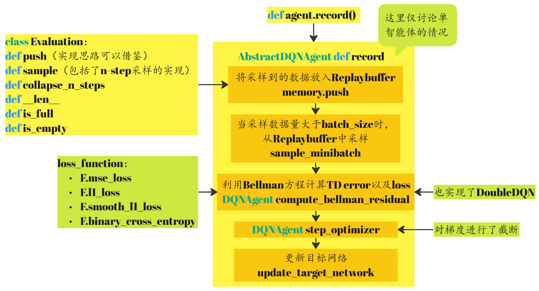
    def record(self, state, action, reward, next_state, done, info):
        """
            Record a transition by performing a Deep Q-Network iteration

            - push the transition into memory
            - sample a minibatch
            - compute the bellman residual loss over the minibatch
            - perform one gradient descent step
            - slowly track the policy network with the target network
        :param state: a state
        :param action: an action
        :param reward: a reward
        :param next_state: a next state
        :param done: whether state is terminal
        """
        if not self.training:
            return
        if isinstance(state, tuple) and isinstance(action, tuple):  # Multi-agent setting
            [self.memory.push(agent_state, agent_action, reward, agent_next_state, done, info)
             for agent_state, agent_action, agent_next_state in zip(state, action, next_state)]
        else:  # Single-agent setting
            self.memory.push(state, action, reward, next_state, done, info)
        batch = self.sample_minibatch()
        if batch:
            loss, _, _ = self.compute_bellman_residual(batch)
            self.step_optimizer(loss)
            self.update_target_network()
Replaybuffer
self.memory是Replaybuffer的一个实现
self.memory = ReplayMemory(self.config)
- push函数的实现可以提升运算速率。
- 在强化学习中,经常需要从经验回放缓存(这里就是
self.memory)中抽样出一批数据来更新模型。而这里的n-step是一个常用的技巧,它表明在预测下一个状态时,不仅仅使用当前的状态和动作,还使用接下来的n-1个状态和动作。当n为1时,这就是常见的单步过渡;当n大于1时,这就是n步采样。
rl_agents/agents/common/memory.py
class ReplayMemory(Configurable):
    """
        Container that stores and samples transitions.
    """
    def __init__(self, config=None, transition_type=Transition):
        super(ReplayMemory, self).__init__(config)
        self.capacity = int(self.config['memory_capacity'])
        self.transition_type = transition_type
        self.memory = []
        self.position = 0

    @classmethod
    def default_config(cls):
        return dict(memory_capacity=10000,
                    n_steps=1,
                    gamma=0.99)

    def push(self, *args):
        """Saves a transition."""
        if len(self.memory) < self.capacity:
            self.memory.append(None)
            self.position = len(self.memory) - 1
        elif len(self.memory) > self.capacity:
            self.memory = self.memory[:self.capacity]
        # Faster than append and pop
        self.memory[self.position] = self.transition_type(*args)
        self.position = (self.position + 1) % self.capacity

    def sample(self, batch_size, collapsed=True):
        """
            Sample a batch of transitions.

            If n_steps is greater than one, the batch will be composed of lists of successive transitions.
        :param batch_size: size of the batch
        :param collapsed: whether successive transitions must be collapsed into one n-step transition.
        :return: the sampled batch
        """
        # TODO: use agent's np_random for seeding
        if self.config["n_steps"] == 1:
            # Directly sample transitions
            return random.sample(self.memory, batch_size)
        else:
            # Sample initial transition indexes
            indexes = random.sample(range(len(self.memory)), batch_size)
            # Get the batch of n-consecutive-transitions starting from sampled indexes
            all_transitions = [self.memory[i:i+self.config["n_steps"]] for i in indexes]
            # Collapse transitions
            return map(self.collapse_n_steps, all_transitions) if collapsed else all_transitions

    def collapse_n_steps(self, transitions):
        """
            Collapse n transitions <s,a,r,s',t> of a trajectory into one transition <s0, a0, Sum(r_i), sp, tp>.

            We start from the initial state, perform the first action, and then the return estimate is formed by
            accumulating the discounted rewards along the trajectory until a terminal state or the end of the
            trajectory is reached.
        :param transitions: A list of n successive transitions
        :return: The corresponding n-step transition
        """
        state, action, cumulated_reward, next_state, done, info = transitions[0]
        discount = 1
        for transition in transitions[1:]:
            if done:
                break
            else:
                _, _, reward, next_state, done, info = transition
                discount *= self.config['gamma']
                cumulated_reward += discount*reward
        return state, action, cumulated_reward, next_state, done, info

    def __len__(self):
        return len(self.memory)

    def is_full(self):
        return len(self.memory) == self.capacity

    def is_empty(self):
        return len(self.memory) == 0
回到record代码中,首先将采样到的数据放入Replaybuffer,当采样数据量大于batch_size时,从Replaybuffer中采样。
    def sample_minibatch(self):
        if len(self.memory) < self.config["batch_size"]:
            return None
        transitions = self.memory.sample(self.config["batch_size"])
        return Transition(*zip(*transitions))
compute_bellman_residual
之后便利用bellman方程进行更新:
loss, _, _ = self.compute_bellman_residual(batch)
    def compute_bellman_residual(self, batch, target_state_action_value=None):
        # Compute concatenate the batch elements
        if not isinstance(batch.state, torch.Tensor):
            # logger.info("Casting the batch to torch.tensor")
            state = torch.cat(tuple(torch.tensor([batch.state], dtype=torch.float))).to(self.device)
            action = torch.tensor(batch.action, dtype=torch.long).to(self.device)
            reward = torch.tensor(batch.reward, dtype=torch.float).to(self.device)
            next_state = torch.cat(tuple(torch.tensor([batch.next_state], dtype=torch.float))).to(self.device)
            terminal = torch.tensor(batch.terminal, dtype=torch.bool).to(self.device)
            batch = Transition(state, action, reward, next_state, terminal, batch.info)

        # Compute Q(s_t, a) - the model computes Q(s_t), then we select the
        # columns of actions taken
        state_action_values = self.value_net(batch.state)
        state_action_values = state_action_values.gather(1, batch.action.unsqueeze(1)).squeeze(1)

        if target_state_action_value is None:
            with torch.no_grad():
                # Compute V(s_{t+1}) for all next states.
                next_state_values = torch.zeros(batch.reward.shape).to(self.device)
                if self.config["double"]:
                    # Double Q-learning: pick best actions from policy network
                    _, best_actions = self.value_net(batch.next_state).max(1)
                    # Double Q-learning: estimate action values from target network
                    best_values = self.target_net(batch.next_state).gather(1, best_actions.unsqueeze(1)).squeeze(1)
                else:
                    best_values, _ = self.target_net(batch.next_state).max(1)
                next_state_values[~batch.terminal] = best_values[~batch.terminal]
                # Compute the expected Q values
                target_state_action_value = batch.reward + self.config["gamma"] * next_state_values

        # Compute loss
        loss = self.loss_function(state_action_values, target_state_action_value)
        return loss, target_state_action_value, batch
with torch.no_grad():用于禁止在其作用域内进行梯度计算- 实现了DoubleDQN
self.loss_function = loss_function_factory(self.config["loss_function"])loss函数包括以下几种:
def loss_function_factory(loss_function):
    if loss_function == "l2":
        return F.mse_loss
    elif loss_function == "l1":
        return F.l1_loss
    elif loss_function == "smooth_l1":
        return F.smooth_l1_loss
    elif loss_function == "bce":
        return F.binary_cross_entropy
    else:
        raise ValueError("Unknown loss function : {}".format(loss_function))
step_optimizer
对梯度进行了截断
    def step_optimizer(self, loss):
        # Optimize the model
        self.optimizer.zero_grad()
        loss.backward()
        for param in self.value_net.parameters():
            param.grad.data.clamp_(-1, 1)
        self.optimizer.step()
update_target_network
更新目标网络
    def update_target_network(self):
        self.steps += 1
        if self.steps % self.config["target_update"] == 0:
            self.target_net.load_state_dict(self.value_net.state_dict())
小结2
到此,整个DQN算法实现完毕,record部分的框图如下:
exploration_policy
这部分主要实现了三种策略:
- Greedy
- ϵ \epsilon ϵ-Greedy
- Boltzmann
此部分可以参考:【强化学习】02—— 探索与利用
Greedy
Greedy贪婪策略即选择最优的策略 a t = arg max a ∈ A Q ( s , a ) a_t=\argmax_{a\in\mathcal{A}}Q(s,a) at=argmaxa∈AQ(s,a)
class Greedy(DiscreteDistribution):
    """
        Always use the optimal action
    """

    def __init__(self, action_space, config=None):
        super(Greedy, self).__init__(config)
        self.action_space = action_space
        if isinstance(self.action_space, spaces.Tuple):
            self.action_space = self.action_space.spaces[0]
        if not isinstance(self.action_space, spaces.Discrete):
            raise TypeError("The action space should be discrete")
        self.values = None
        self.seed()

    def get_distribution(self):
        optimal_action = np.argmax(self.values)
        return {action: 1 if action == optimal_action else 0 for action in range(self.action_space.n)}

    def update(self, values):
        self.values = values
ϵ \epsilon ϵ-Greedy
ϵ
\epsilon
ϵ-Greedy公式如下:
a
t
=
{
arg
max
a
∈
A
Q
^
(
a
)
,
采样概率:1-
ϵ
从
A
中随机选择
,
采样概率:
ϵ
a_t=\begin{cases}\arg\max_{a\in\mathcal{A}}\hat{Q}(a),&\text{采样概率:1-}\epsilon\\\text{从 }\mathcal{A}\text{ 中随机选择},&\text{采样概率: }\epsilon&\end{cases}
at={argmaxa∈AQ^(a),从 A 中随机选择,采样概率:1-ϵ采样概率: ϵ
这里实现的其实是衰减贪心策略,衰减曲线如下图所示。
ϵ
=
final-temperature
+
(
temperature
−
final-temperature
)
∗
e
−
t
τ
\begin{aligned}\epsilon &= \text{final-temperature}+(\text{temperature}-\text{final-temperature})*e^{\frac{-t}{\tau}}\end{aligned}
ϵ=final-temperature+(temperature−final-temperature)∗eτ−t

class EpsilonGreedy(DiscreteDistribution):
    """
        Uniform distribution with probability epsilon, and optimal action with probability 1-epsilon
    """

    def __init__(self, action_space, config=None):
        super(EpsilonGreedy, self).__init__(config)
        self.action_space = action_space
        if isinstance(self.action_space, spaces.Tuple):
            self.action_space = self.action_space.spaces[0]
        if not isinstance(self.action_space, spaces.Discrete):
            raise TypeError("The action space should be discrete")
        self.config['final_temperature'] = min(self.config['temperature'], self.config['final_temperature'])
        self.optimal_action = None
        self.epsilon = 0
        self.time = 0
        self.writer = None
        self.seed()

    @classmethod
    def default_config(cls):
        return dict(temperature=1.0,
                    final_temperature=0.1,
                    tau=5000)

    def get_distribution(self):
        distribution = {action: self.epsilon / self.action_space.n for action in range(self.action_space.n)}
        distribution[self.optimal_action] += 1 - self.epsilon
        return distribution

    def update(self, values):
        """
            Update the action distribution parameters
        :param values: the state-action values
        :param step_time: whether to update epsilon schedule
        """
        self.optimal_action = np.argmax(values)
        self.epsilon = self.config['final_temperature'] + \
            (self.config['temperature'] - self.config['final_temperature']) * \
            np.exp(- self.time / self.config['tau'])
        if self.writer:
            self.writer.add_scalar('exploration/epsilon', self.epsilon, self.time)

    def step_time(self):
        self.time += 1

    def set_time(self, time):
        self.time = time

    def set_writer(self, writer):
        self.writer = writer
Boltzmann
玻尔兹曼分布(Boltzmann Distribution)是描述分子在热力学平衡时分布的概率分布函数。它表明在给定的能量状态下,不同的微观状态出现的概率是不同的,且符合一个指数函数形式。
在热力学中,任何物质在一定温度下都会具有一定的热运动,这些热运动状态可以用分子内能或动能来描述。而玻尔兹曼分布表明了在相同温度下,分子在所有可能状态之间的分布概率。其表达式为:
P ( E i ) = e − E i / k T ∑ j e − E j / k T P(E_i) = \frac{e^{-E_i/kT}}{\sum_{j} e^{-E_j/kT}} P(Ei)=∑je−Ej/kTe−Ei/kT
其中, P ( E i ) P(E_i) P(Ei)为分子处于能量状态 E i E_i Ei的概率, k k k为玻尔兹曼常数, T T T为温度, E j E_j Ej为所有可以达到的能量状态。
可以看到,玻尔兹曼分布中每个能量状态的出现概率与其能量成负指数关系,因此能量较小的状态出现的概率更大。这符合熵增加的趋势,即越有序的状态出现的概率越小。
class Boltzmann(DiscreteDistribution):
    """
        Uniform distribution with probability epsilon, and optimal action with probability 1-epsilon
    """

    def __init__(self, action_space, config=None):
        super(Boltzmann, self).__init__(config)
        self.action_space = action_space
        if not isinstance(self.action_space, spaces.Discrete):
            raise TypeError("The action space should be discrete")
        self.values = None
        self.seed()

    @classmethod
    def default_config(cls):
        return dict(temperature=0.5)

    def get_distribution(self):
        actions = range(self.action_space.n)
        if self.config['temperature'] > 0:
            weights = np.exp(self.values / self.config['temperature'])
        else:
            weights = np.zeros((len(actions),))
            weights[np.argmax(self.values)] = 1
        return {action: weights[action] / np.sum(weights) for action in actions}

    def update(self, values):
        self.values = values
运行结果
运行命令与方法在上一讲已经介绍【rl-agents代码学习】01——总体框架。
超参数设置采用默认设置,使用DQN算法分别运行4000steps和20000steps。使用Tensorboard查看结果:
tensorboard --logdir C:\Users\16413\Desktop\rl-agents-master\scripts\out\IntersectionEnv\DQNAgent\baseline_20231113-123234_7944\
4000steps


可以看到最后的episode reward大致在3左右。
20000steps

可以看到最后的episode reward大致在3左右。